I’m not quite sure where this belongs, I guess I’ll post it here.
Why are you posting a suggestion here? The developers are unlikely to see it. If you really like it so much, why don’t you show your support by implementing it yourself, or at least donating to show you care? If you can’t contribute more than an idea, please get out.
That’s just not really an option for me. I know, it hurts my credibility. But I hope the idea may make its way to someone who can make it happen.
What makes you think your idea hasn’t been suggested before? If it’s some obscure new feature nobody will use, what reason do the developers have to implement it?
I’m suggesting something which already exists outside of Blender but which is rather unpopular. I know Blender can push new standards. It can make a good idea popular by supporting it.
So now, onto the actual suggestion.
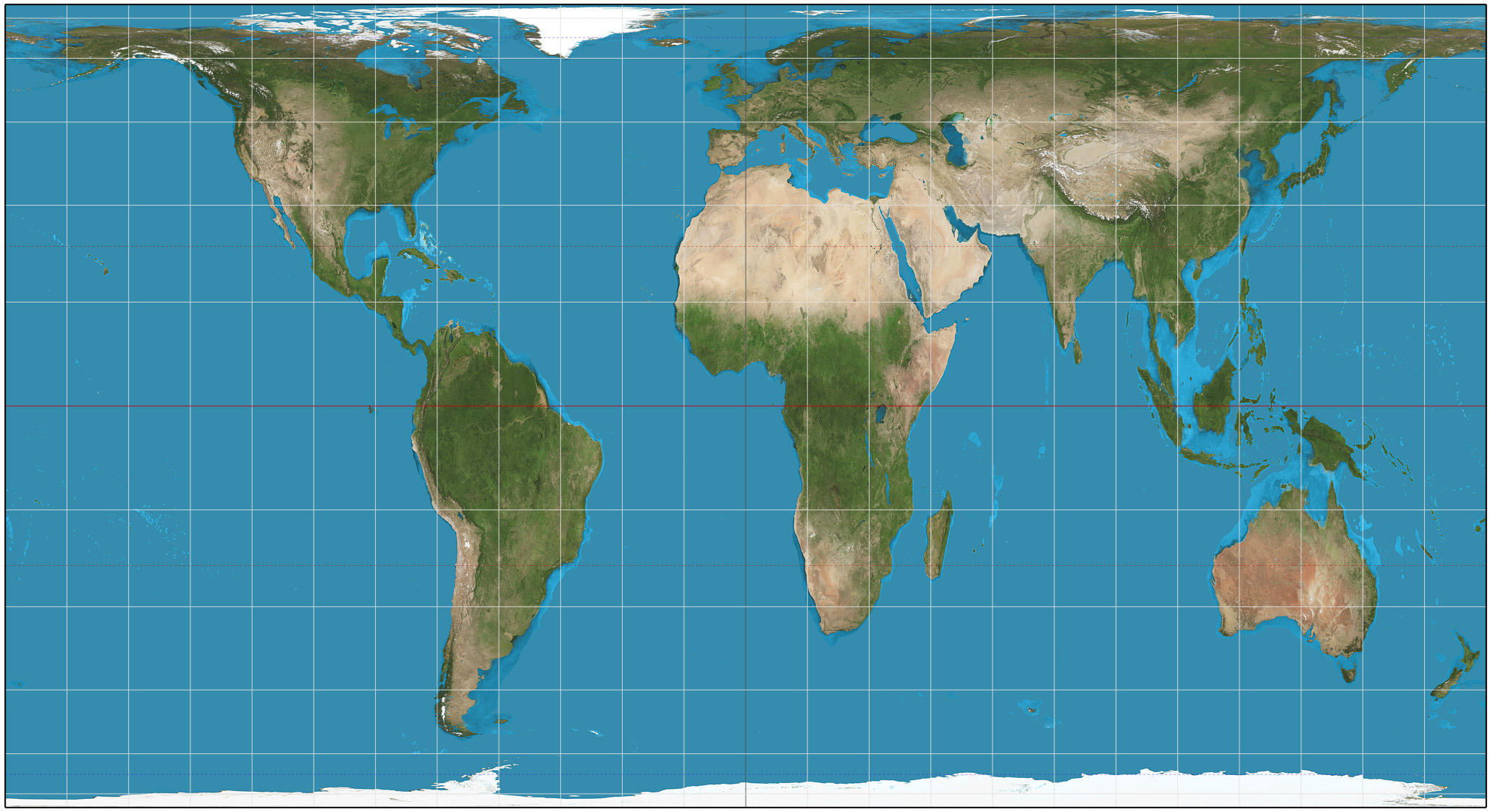
The current popular method for environment textures is the equirectangular projection. In the equirectangular projection, the (θ, φ) from the spherical polar coordinates are directly mapped to (X, Y), with scaling as needed.
The equirectangular projection scales all slices of the sphere to the same size rows in the texture. This results in the tiny slices near the poles using up as many pixels as the equator, even though the equator makes up much more of the view. The poles have an extreme amount of detail, while the equator gets less.
This distribution of detail is very bad. As artists, we want our textures with high enough resolution to ensure a minimum amount of detail everywhere, and we will end up using large textures just so the equators have enough detail, while the poles are using a disproportionate amount of pixels and have far more detail than we need.
We have some primary goals here when choosing a projection:
- Even distribution of detail.
- Low distortion.
- High performance.
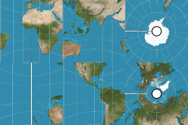
I propose the cube projection. It is constructed by taking the unit sphere and projecting it from the origin onto the unit cube. This results in one component of the vector always being -1 or 1, while the other two range between -1 and 1. We take the squares which are the cube faces, and arrange them in a 3x2 grid like so:
We lay them out in a grid instead of as a cube net. A cube net wastes space in the image, as there are large regions which do not encode data anywhere on the sphere. It also results in slightly worse performance since some squares need to be rotated to become the proper cube face and the rotation is different for each face, requiring either branching or a complicated bit twiddling sequence. The cube net needs special code for seam handling anyway, so it is not a problem that my proposed layout also has seams to deal with.
Before implementation details, consider why a cube projection has better distribution of detail and low distortion. The centers of the faces are touching the unit sphere, so the scaling here is 1. At any point on the cube which is angled θ to the normal axis, the scaling is tan’(θ) = sec(θ)² on the axis joining the face center and the point on the face, and sec(θ) on the perpendicular other axis on the face, for a scaling factor of sec(θ)³. At any point on the cube which is distance r from the origin, the angle to the normal axis is θ = arcsec®. Thus the scaling at that point is sec(arcsec®)³ = r³. At the edge center, this is (√2)³, so we use around 2.8 times as many pixels to cover the same amount of visual space. At the corners, this is (√3)³, so we use around 5.2 times as many pixels to cover the same amount of visual space. It cannot get more extremely scaled than the corners, so we have an upper bound of √3³. We established the lower bound of 1 before, at the center. At worst, the cube projection produces √3³ times as much detail at one point compared to another, this is a great improvement from the equirectangular projection which has no upper bound on the detail, since the slice nearest to the pole can be arbitrarily small compared to the equator and thus pack the pixels infinitely tight. As for distortion, we need to divide the scaling factors instead of multiplying them, which results in sec(θ)²/sec(θ) = sec(θ) = sec(arcsec®) = r, at worst, √3. As a sanity check, here is the adjusted area of a cube face, which is 1/6 of the unit sphere’s surface area as expected.
Now for practical implementation details.
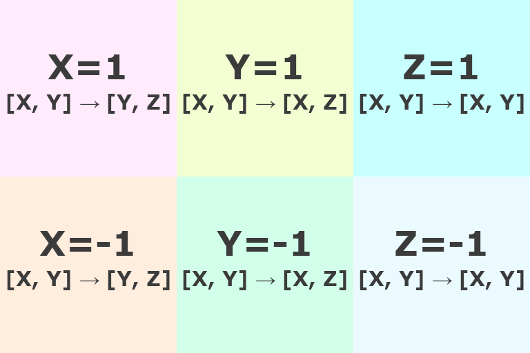
The free two axes correspond to the two image axes, for example, in the [X=1] square, the [X, Y] axes in the image get mapped to [Y, Z] axes in the projection. The squares themselves are ordered as X, Y, Z. There is no particular reason for these choices, other than they are the most straightforward, since another permutation could not hurt performance much.
As for why the …=1 is above and …=-1 is below, this choice is explained by the image format and the IEEE 754 floating point format. Images are stored conventionally with +Y being down instead of up. If we floor divide the y position in the image by half the image height, we will get 0 for the top row of squares and 1 for the bottom row of squares. Alternatively, we may see if the y position is greater than or equal to half the image height, which is 0 (false) for the top row of squares and 1 (true) for the bottom row of squares. In a standard floating point number, 0 as the sign bit means positive and 1 as the sign bit means negative. Is flipping one bit that big of a deal for performance? No. And it would feel silly to call this a performance optimization. It’s possibly one less instruction, maybe not even. But the existing floating point specification is a convenient tiebreaker here.
A possible complaint is that some squares will be flipped, since no rules for maintaining orientation are forced in this projection. Keep in mind that the cube projection is a representation of data on a sphere, so you really should be looking at the sphere and not the flat projection.
There is also the cylindrical equal area projection. It has the same detail level everywhere, and it is not that computationally expensive. What do you think cube projection would do better than it?
Both cylindrical equal area projection and equirectangular mappings create a lot of distortion. It is still an image we are trying to display as an environment map, and if the pixels are heavily skewed along some axis it makes it difficult to represent some objects accurately. Cube projection has a lot less distortion.
It’s a bit unfair to be throwing in a third goal of minimizing distortion now. It’s like I added that in specifically to make cylindrical equal area projection look bad. It is bias on my part, I admit, I just like cube projection more, but I can still have a civil discussion about it. This is for the improvement of Blender after all, there’s no reason we can’t have both.
Here is a brief comparison:
Cube projection:
- √3³:1 most extreme detail ratio (center vs corner)
- √3:1 most extreme distortion (center vs corner)
- has several cuts, squares need to be stitched together correctly, needs special texture handling to avoid incorrect interpolation and artifacts at cube edges
- involves square root in computation
- based on Cartesian coordinates
Cylindrical equal area projection:
- 1:1 most extreme detail ratio (completely uniform)
- ∞:1 most extreme distortion (equator vs poles)
- sides need to loop but poles need to not loop, so needs special texture handling to avoid incorrect interpolation and artifacts at poles
- involves trigonometry in computation
- based on cylindrical polar coordinates
I don’t think I’m qualified to do more detailed comparison.
I know some people will want to see what cube projection would look like. I don’t actually have a setup for it, so I took the map of Earth and applied some image warping to get this mockup. I’m very confident I screwed up the axes, so please don’t rely on it as a reference.