Having fun with geo nodes-based particle simulations in this little weekend project, exploring curl fields in the process.
Sound design in Ableton.

Quick breakdown:
- The emitters are simply animated by setting their position based on a combination of sine/cosine functions driven by the scene time
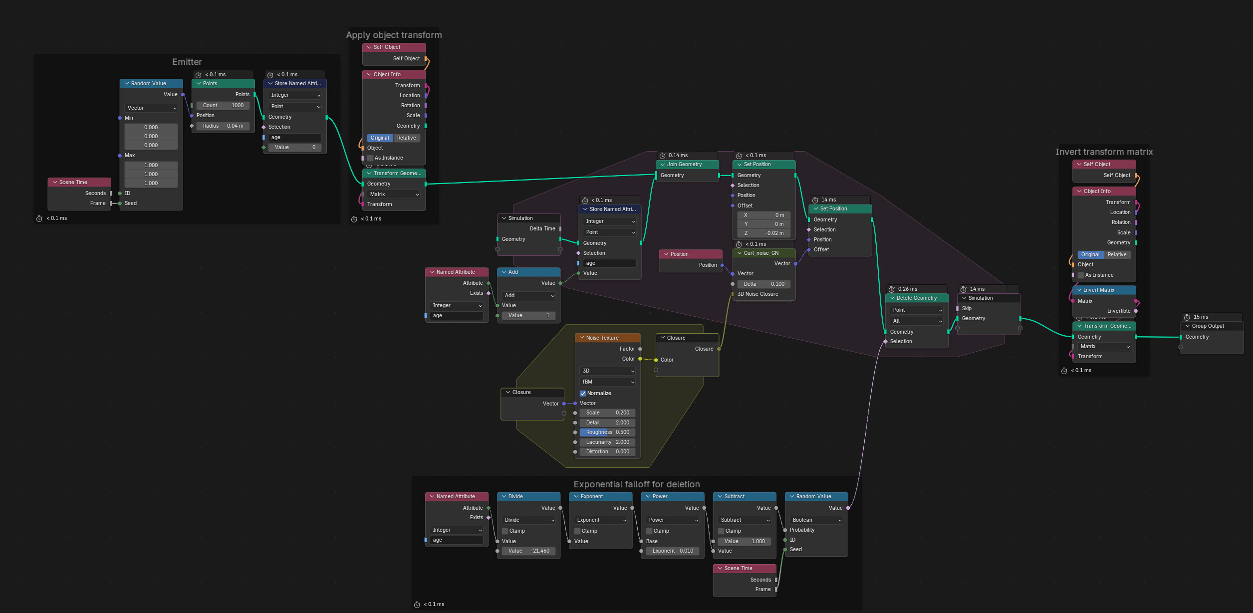
- Points are distributed on the faces of the emitters, and joined into a simulation zone:
- Inside the sim zone, we update the particle positions according to the curl noise
- We update the particle age (needed for shading and deletion)
- Particles are deleted with a probability that increases by particle age

Wtf is a curl noise?
It’s easy to get too deep into vector math here, but let me try to keep it simple.
Let’s say you’ve got a scalar 2D perlin noise on a plane (aka the Factor output of your run-of-the-mill noise node). Now imagine you’re using that value to displace the plane upwards to create a landscape. The gradient field of this scalar field would then be the set of directions that point towards the steepest incline at each point on the plane. If you moved your particles along this gradient field, you’d end up collecting all particles on the top of the hill (not what we want). This is type of field has sources and sinks, meaning there are places where either no particles can ever be, or where all particles end up chilling.
In fluid dynamics, you deal with divergence-free fields, without sources or sinks. Translated to our landscape, we’d have to create a vector field that gives us the directions along the slope instead of up or down. In 2D, it’s as easy as calculating the cross product between the vector facing away from the plane (Z) and the gradient (aka rotating around 90° along Z). Congrats, you’ve got yourself a 2D curl field!
Here’s an example. If you moved your particles directly along the gradient, you’d get this:
But with a curl field, the particles end up looking like pollen on a lake, and their relative distances remain mostly constant:
Now the hard part is imaging this in 3D space instead. There is no “up”, since “up” is just another dimension of the scalar field.
Luckily for us, smart people already did the thinking for us: https://www.cs.ubc.ca/~rbridson/docs/bridson-siggraph2007-curlnoise.pdf
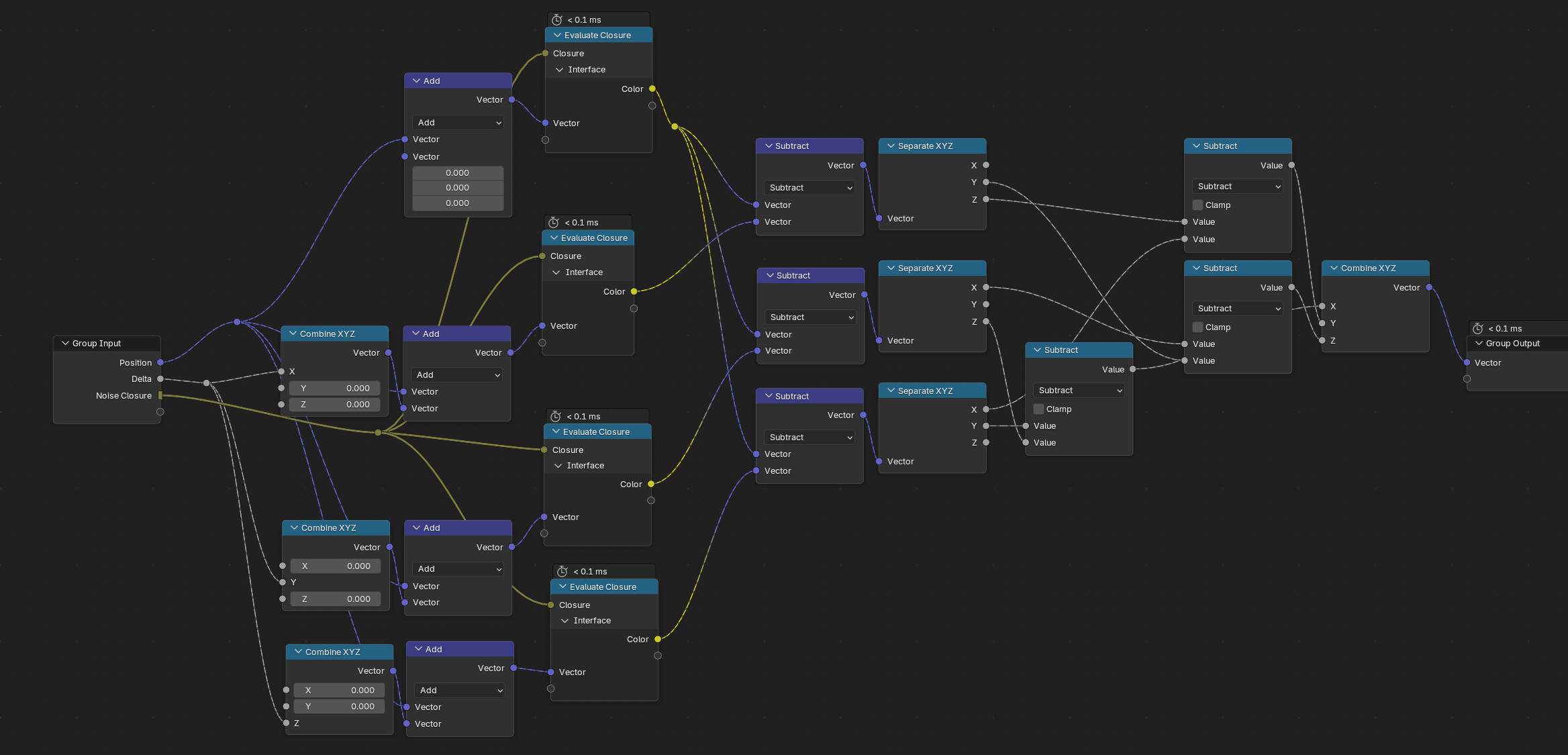
Translating these formulae into geo nodes gives us this setup:

In essence, we first calculate the partial derivatives (the rate of change in each of the three dimensions), for which we need to offset the 3D noise by a delta value. The resulting vectors are then connected according to:

As delta, we take a small step size (between 0.01-0.1 maybe), and as output we get a vector we can use as offset for each particle inside the simulation.
Give it a try, its quite simple! No computationally expensive boid simulation needed. On my laptop, this still runs in real-time (~30fps) with close to 30k particles.