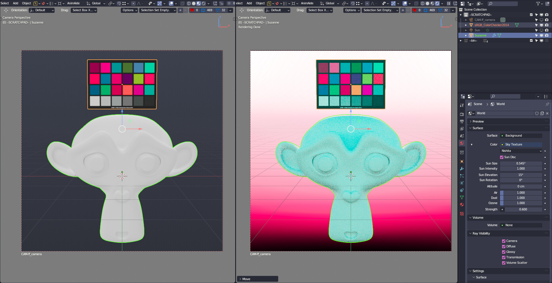
Can you share the .blend file? Because I am unable to reproduce the issue with my own files.
It really is just a random image i used. It also affected any external image or sky texture (Light object and preview HDR doesn’t get affected). I think it’s also affected the standards and guard rail, but it really noticeable in AgX with higher contrast looks
test.blend (4.7 MB)
If you can’t reproduce it on your files, maybe there’s a difference between your config and the one in gitea? i downloaded the file manually one by one (except the content in filmic folder because it doesn’t get updated since the last time i downloaded it)
I just redownloaded from Gitea and I still cannot reproduce:
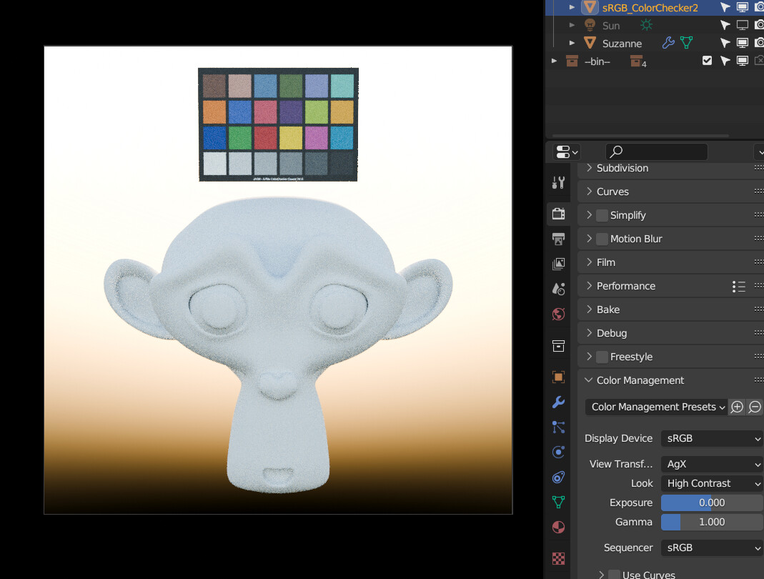
Maybe you can try redownloading, maybe something went wrong during the download.
I wouldn’t download each file one by one, what I did was downloading the entire branch first:
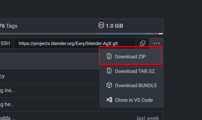
The zip file is only 75.27 MB, not very large.
After downloading, in the unzipping program, we can select the colormanagement folder, and only unzip that folder.
That’s what I do every time. No need to download each file individually.
1 Like
Ah you’re right, i thought the size would be higher similar to blender zip file so i didn’t checked it.
Yes the issue is gone once i downloaded it, maybe just some corrupt file (kinda strange because it never happen before).
Thanks!
*edit: i think i know where the problem is, it is because I’ve made a mistake when modified the config to add Adobe RGB, now that i’ve checked the config file again, the manually downloaded one is also didn’t have any problem
I’ve been looking into gradient domain solutions for something that is vastly closer to visual cognition than the absolute nonsense of discrete sampling approaches.
I figured folks who are mathy math types (hello @kram10321, among some of the other wise lurker minds) might find these rather insightful.
The elegance of a gradient domain theory is that such an approach is likely much closer to our visual cognition mechanics. Such an approach also removes the discrete sample issues with negatives and the foolish relative-absolute colourimetric thinking.
I am pretty much fully brain wormed into relational field thinking at this point when it comes to visual cognition, so YMMV if you are not quite as lost in these woods as I am. As with all bits of attaching maps to territories, the domains matter much. If folks were looking for a hint as to what could be most potentially useful as an underlying domain metric, I would suggest something that is broadly congruent with the signals in the Lateral Geniculate Nucleus. That is, something that would be a reasonable underlying uniform signal would be something that peels the process into an opponency based set of magnitudes:
- RGB to CIE XYZ.
- CIE XYZ to PDT (aka LMS)
- PDT to
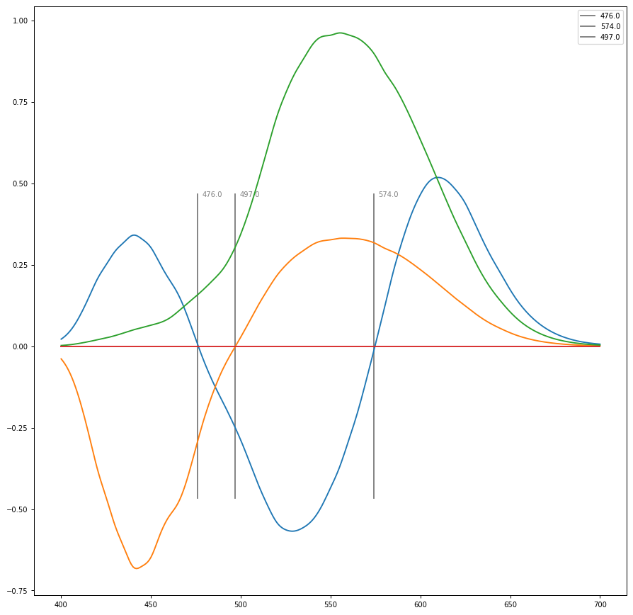
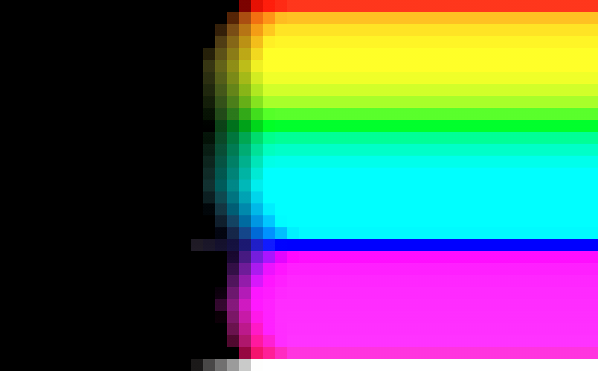
(P+D),(P+-D),(P+D)+-T. EG Orthogonal combination of the three visual channels or D. B. Judd’s Response Functions for Types of Vision According to the Muller Theory. The tell as to whether or not the weightings are reasonable will be whether or not there’s a crossover at ~575nm. If the weightings are reasonable, you should see something similar to the following null crossovers. I place heavy emphasis on those broad crossover points as there are other pieces of visual cognition research that are congruent with them, such as that from Thornton, Houser, Smet, Esposito, and many, many others.
Using the above, coupled with the general gradient approaches outlined in the following documents, might end up with something that is a fresh approach that could offer a much more forward looking approach to the problem at hand.
Space-Dependent Color Gamut Mapping: A Variational Approach
Color Gamut Mapping Based on a Perceptual Image Difference Measure
5 Likes
@troy_s @Eary_Chow Can you guys explain what the difference is between ‘Eary’s AgX Version 12.3 RC’ and the original ‘AgX’ from Troy’s GitHub? Besides the different ‘Looks’, is there anything else happening under the hood when it comes to image formation, whereby the produced image looks different? I’m asking because ‘Eary’s AgX Version 12.3 RC’ doesn’t work on some programs, like Affinity Photo 2, while the original AgX does, so I’m wondering if I can use them both if they produce the same results, as far as the base look transform is concerned.
Again my version uses a lot of OCIOv2 features, while a lot of DCCs are not catching up to V2. As someone has comfirmed in one of the previous posts, it seems Affinity doesn’t have OCIOv2 support yet.
The contrast looks used Grading Primary Transform, an OCIOv2 feature. My version packs the two power curve spaces to the named transforms, which is also an OCIOv2 feature. My version uses some new OCIOv2’s new builtin transforms, etc. There are just a lot of differences.
My version is updated with the discussion happened in this thread, as well as some of my own designs (like the CIE-XYZ I-E reference space).
Troy actually has several different AgX repos, but I assume you are talking about the original one that hasn’t been updated for more than a year. That was the original proof of concept version before all the discussions in this thread. Troy also has a newer python script version and a Resolve DCTL version, but I think most people are still talking about the original proof of concept version.
3 Likes
What’s the difference between 12.3 RC and the Gitea version?
Visually, there is a difference but I missed the exact changes
Gitea version recently got a LUT precision boost for the Guard Rail.
Oh, I guess that info should be spread better.
I think people are still downloading 12.3 RC right now
It’s not a huge deal, I still expect the Gitea version to be merged shortly, then we don’t need to worry about people downloading.
The Gitea version is still not settled regarding the Filmic Looks though. I asked Brecht about it in the last Cycles meeting, he said he would still like Filmic Looks to be supported even in 4.0. He said the required code change “shouldn’t be too difficult” though, I hope it can be done soon. (He also mentioned he didn’t have time to do a proper review though, let’s hope things go smoothly.)
6 Likes
do we have somebody on the case yet for the Blender-side development?
As said, I don’t think Brecht did any such thing as to promise that would be done by him. Somebody has to step forward to actually do that
1 Like
I don’t have time right now to read those various links so it’s very likely that one of them might be answering my question anyway, but how would this be used?
If I understand right from your explanation, this amounts to transforming to a different color space of sort, perhaps a perceptual space, where each axis is orthogonal, and some reasonably-ranged values are going to involve negatives?
It’s in its nature also somehow more relational?
So could you just, say, “do AgX” in that space and then transform back? - Except AgX is specifically geared right now towards positive values. You’d need a different type of compressor. Perhaps one that doesn’t move black at all but compressed large negative values to something like -1 and large positive values to something like +1
How do you deal with logarithmic values then?
Or are you talking about a completely different thing here?
I think it will be done by him, he did some similar thing back in 2.79 anyways, and he didn’t quite make it clear what the “code change” is specifically referring to, “code change” is quite a vague word, if he is not planning to do it himself, I would expect him to be more specific about it, instead of going with “code change”. Though he did mention in the Cycles meeting it’s a view transform based filtering, I think it comfirms it’s something similar to the filtering back in 2.79.
I think the exact opposite: If he were planning on doing it, he’d explicitly say so.
I’m sure he’d answer a question about what specific code would have to be changed though
1 Like
The broad concept is essentially following Claude Shannon, and later Dennis Gabor. Specifically, that there are effectively two extrema of projections of a signal that we can interact with:
- Discretized Samples.
- Frequency.
Gabor refined this stance and provided the uncertainty principle. That can be loosely explained that as we leave the discrete samples projection, and trend toward the frequency representation, that we lose the information of the other. TL;DR: When we are fully in the discrete samples projection, we have no information of the frequency, and when we are in the frequency projection, we have no information of the spatial orientation.
So what the hell does any of this have to do with potential areas for experimenting?
I’d probably suggest that every single manipulation can be tackled from a fields-first / frequency domain approach.
Specifically in relation to this thread, we have quite a few discussions about posterization, and how it manifests for example. The transformation of values from one additive projection to another poses quite a few problems here. We can outline that:
- The manifestation of posterization is not within an evaluation of the discrete magnitudes. That is, given sample A to sample B, the posterization is neither in A nor B, but in the relationship C between the two.
- The analysis of posterization is uniquely cognitive; there’s no analysis of graphs or magnitudes that anyone is able to look at to suggest where trouble may be.
- The spatial sample resolution is intimately tied to the experience of posterization in the formed picture, and there is currently no method to predict what zoom size etc. affords us any utility in diagnostic analysis.
Effectively we have what amounts to random approaches of f*cking fish for any of the above insights.
I am going to outline what led me here, and why I think that image manipulations, across all manifestations, could profoundly benefit from a field relationship first line of thought. Ideally this leads to some experimentation.
The demonstration here will focus on one of the classical Cornsweet, Craik, O’Brien demonstrations. I have chosen this one as it varies solely in luminance, to help us reduce the dimensionality complexity. In terms of articulation, it varies strictly in the horizontal dimension, which helps us reduce the dimension projection of the plots.
Let’s take a look. Note that we should exert some caution with respect to our visual field, as at a given zoom level, or distance from your device, the colour cognition will vary. For example, zooming in to a specific region will shift the spatiotemporal field articulation presented to us, and may amplify or attenuate the cognitive result.
Here’s the basic demonstration image in question.

First, let’s plot the luminance, in uniform luminance units, across this picture.
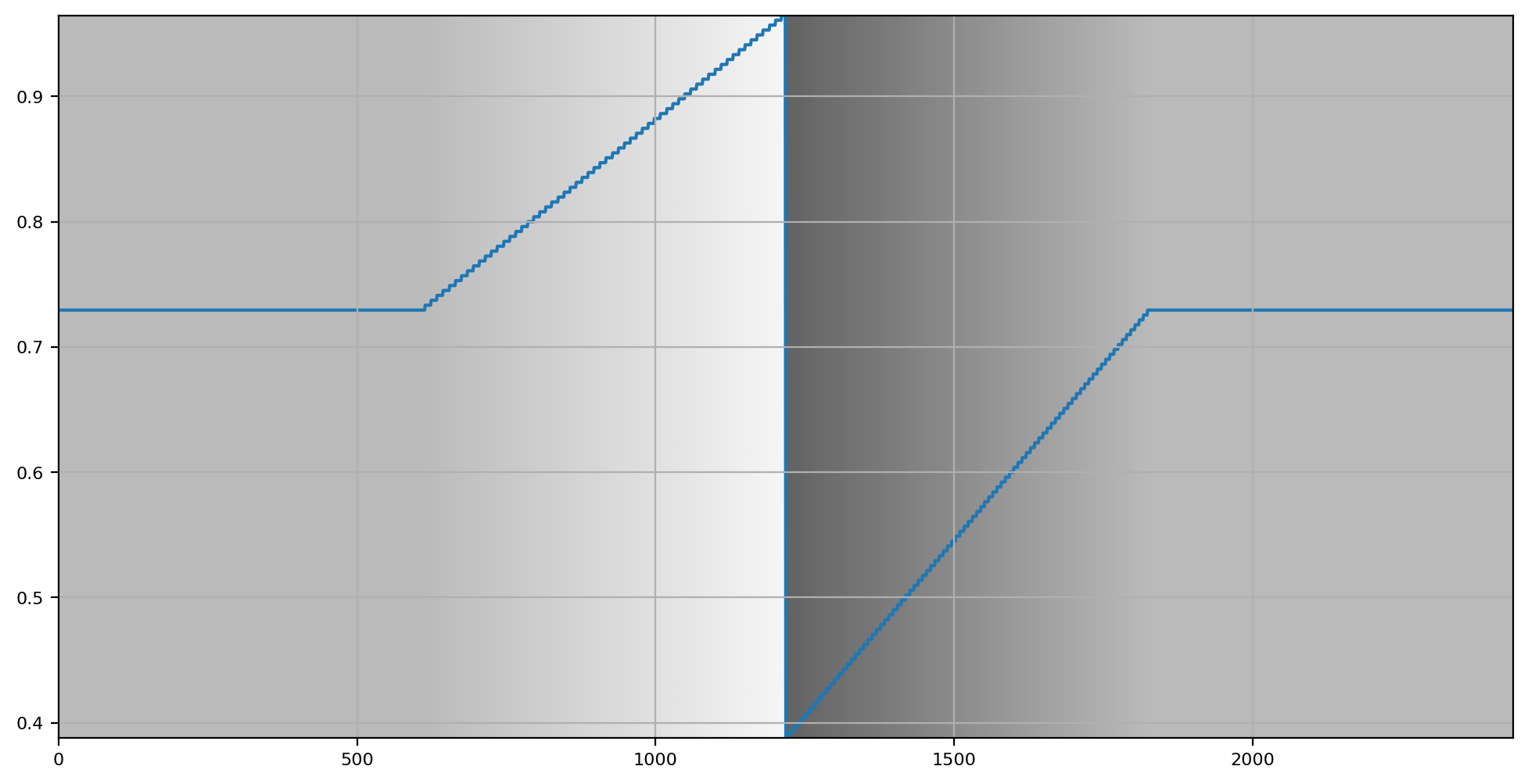
As we can see, the plot indicates that the increment in colourimetric luminance in the gradient is uniform. Further, we can also see that the luminance of the non-graduated regions on the left and the right are constant, and of identical tristimulus magnitude.
I’d like to focus on two specific cognitive results here:
- The broad cognition that the left region appears lighter than the right region.
- The more nuanced dip that forms immediately adjacent to the gradients on either side.
That is, the cognition of the picture is rather disconnected from the tristimulus magnitudes. No amount of discrete sampling of the values will provide us with any insight. Let me remind ourselves that the discrete samples thinking is purely one end of the Shannon information signal theory. Let’s look at the other end… the frequency domain.
Here, I’ve chosen a very low frequency octave. It’s simply a wide “blur” that is compared against the unblurred values if you will. We’ve shifted from the spatial sampling domain, to the relational frequency domain.
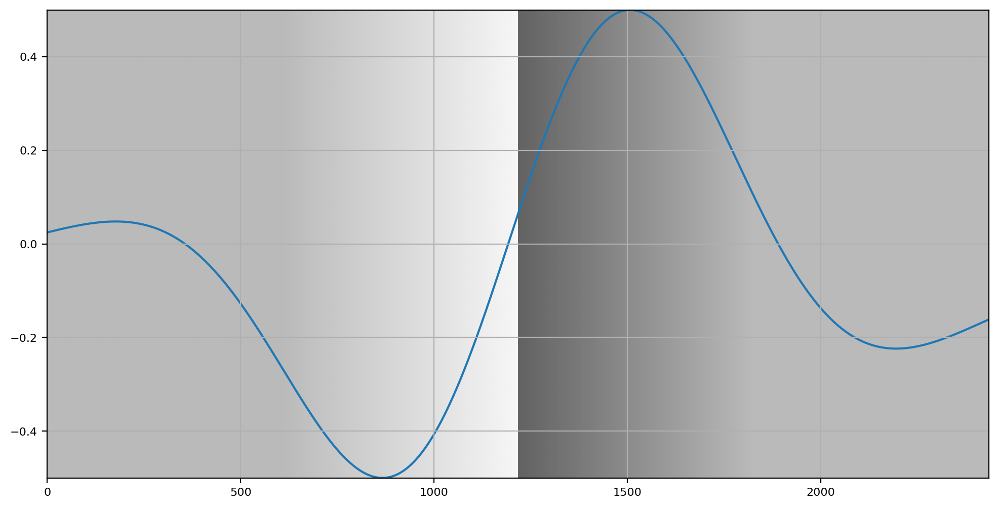
Note how the graph broadly approximates the cognitive impact of the left to right “lightness” versus “darkness” relationship. On the left, the frequency analysis lifts above the magnitude of the discretized samples, and the right side dips below the sampling representation. We are already manifesting something that is closer to our cognition of the picture than anything we can derive directly from the samples end of the Shannon signal.
Now let’s analyze a higher frequency representation. Not quite the highest frequency, but a partial octave down.
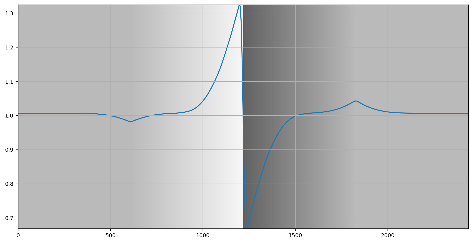
Yet again we are able to see a direct connection between the colour cognition and the representation.
Now while these demonstrations are rather simplistic, we should not overlook how complex the visual cognition of the spatiotemporal articulations are. Given that I’ve seen exactly zero approaches out in the commons that present a viable mechanic to predict the amplification / attenuation of the picture signal, I’d hope that folks here can appreciate the rather profound implications of shifting our projections away from sampling, and toward frequency analysis.
And of course the examples above are carefully chosen. When dealing with an achromatic signal, there’s a happy congruency where when R=G=B, we are strictly dealing with luminance. We know that in terms of our visual cognition pathways, specifically the signal that is transmitted along the Lateral Geniculate Nucleus routing, that there happens to be a signal that seems highly correlated to what we’d describe as a luminance magnitude. Granted, if our visual cognition is heavily frequency analysis based, no fixed function is possible, as the signal is frequency relational defined, not samples based! As such, we should expect that no samples based magnitude is “ideal”, but it’s the best we have. We should be able to agree that there’s some incredible correspondence here, even if the underlying Map to Territory relation between the magnitude of a value and the territory we are seeking to describe is potentially less than idealized.
So where does this leave us?
Let’s reconsider the three points I raised above:
- The manifestation of posterization is not within an evaluation of the discrete magnitudes. That is, given sample A to sample B, the posterization is neither in A nor B, but in the relationship C between the two.
- The analysis of posterization is uniquely cognitive; there’s no analysis of graphs or magnitudes that anyone is able to look at to suggest where trouble may be.
- The spatial sample resolution is intimately tied to the experience of posterization in the formed picture, and there is currently no method to predict what zoom size etc. affords us any utility in diagnostic analysis.
We have hopefully seen that by shifting the projection from sampling to frequency, we have an avenue to approach an analysis domain projection of 1.
If we think about posterization as being a discontinuity of the relationship between samples, where the continuity is evaluated in the frequency projection, and we have a reasonable magnitude domain for analysis, we might have a potential avenue for evaluating posterization in pictures formed to make progress on 2.
Finally, we can couple 1 and 2 with the idea of a viewing field frustum to evaluate 3. That is, while the demon is in the details, a broad strokes evaluation of samples per spatial dimension, derived from a basic frustum calculation, could help us calibrate the evaluations for 1 and 2 in determining thresholds for posterization.
For example, for broad strokes picture formation, I believe we could take the above general principles and apply them to some of the sweep patterns. That is:
- We could create sweeps with specific attention to targeted quantisation levels.
- We could create sweeps with “surrounds” that match varying surrounds to account for reader contexts.
- We could analyze the sweeps to back project curves that drive the picture formation to optimize for reducing general posterization.
- We could analyze the gradient domains of a wider gamut projection, for example Display P3, to match the gradients and solve for a more idealized gamut projection into BT.1886 / sRGB.
Again, I stress, the domain of the magnitude is critically important here. I don’t believe we will gain anything evaluating the frequency of RGB for example, given that we know the biological signals are rather different. I have been leaning more and more strongly toward an LGN-centric three component model. I’ve had good results broadly predicting both the achromatic and the chromatic cognition present in the following pictures, for example:


Now where this gets even more interesting is if we shift our entire vantage of picture manipulation and production away from the sampling thinking, and toward frequency.
When we think about what image authors need, we have broad concepts like:
- “I’d like to increase the chroma of this region to make the colour pop.”
- “I want to increase the overall contrast of the image.”
- “I’d like to reduce noise in the formed picture.”
- “I’d like to subtly draw the reader’s eye to a region of the picture.”
- “I’d like to counter the Abney effect in this region.”
- “I’d like to reduce the posterization in this region.”
All of the above are a direct line to a fields-first projection of the problems, and are potentially much more aligned with visual cognition when addressed in the frequency, or hybrid Gabor frequency domain.
Hope this helps clarify where we might be able to take the concepts. I know there are some incredibly wise lurkers to this thread. I hope that I’ve managed to at least provide a bit of evidence that there’s an absolutely massive series of gains sitting in these sorts of concepts. The concepts have been around forever, but haven’t quite hit mainstream image authoring tools in force, sadly.
13 Likes
Do these need to replace the old ones (standard & filmic), can’t they just be added as new options? Unless its similar, but more useful, and can reproduce exactly the old result.
I did some testing with local tone mapping from papers quite a long time ago and the way it increased local contrast seemed really useful. A modern version of that would be nice to have as tone mapping option.
1 Like
The Gitea version already has these two back in the view transform manu, as requested by Brecht.
I am still not sure what an “ultimately ideal” local “tonemapper” should produce in the case of the sweep EXR, as visually you still need to have cue for “brightness change”, brighter areas shouldn’t look the same as darker areas, otherwise you will see clippings and skewings. I am not sure whether “local tonemapping” is the correct direction.
Maybe you can test these “modern local tonemappers” with the said sweep EXR and see if they produce results that visually make sense. If the results don’t make sense, it’s probably not a good idea.
1 Like
I ran the sweep image through my implementation of a 2004 paper for you:
This is using parameters that give decent results for photos.
And… as you can see in your result, it doesn’t have visual cue for which part of the image is brighter, it clips all the way through