Shader Node Matrix Operations

[kram10321]

I figured it might be useful for people to have access to matrix operations in shader nodes.

These could be used for a variety of use cases including manually converting between color spaces or working in specific or randomized coordinate frames.
Pretty much all of this should also be translatable right into Geometry Nodes if you need anything of the sort there.

First things first: How to bring a matrix into Blender’s shader nodes?

Let’s start with the most obvious case, the 1×3 matrix, aka a column vector:

Column Vector in ℝ^1×3

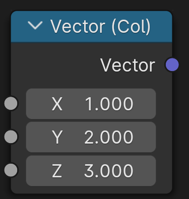
The vector

1
2
3

From there, it’s easy to add extra columns:

A 3×3 matrix is just a collection of three column vectors:

Matrix in ℝ^3×3

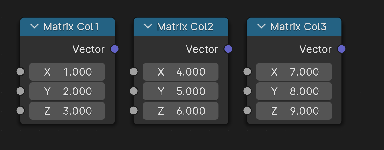
This represents the matrix

1 4 7
2 5 8
3 6 9

A fundamentally important matrix 𝟙 which is the unit matrix. It has the properties:

• 𝟙 v = v
• 𝟙 M = M
• M 𝟙 = M
• 𝟙² = 𝟙^-1 = 𝟙

and simply looks like this:

Unit Matrix 𝟙₃ in ℝ^3×3:

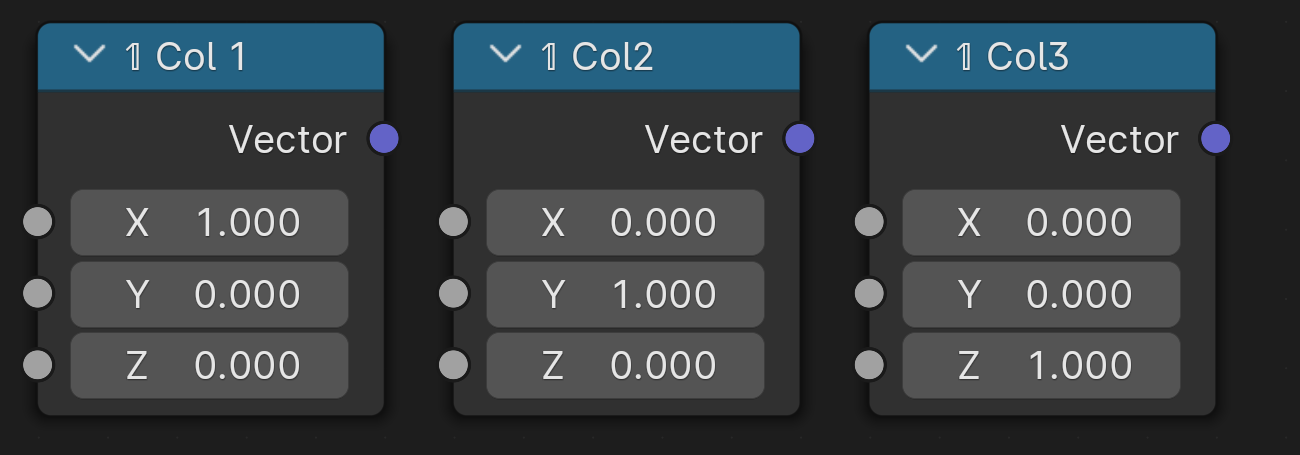
It’s called the unit because it acts like the number 1 does for regular numbers. It’s basically a no-op.

---

And now, let’s define some fundamental operations on matrices:

• multiplication M v or M N — applying M to v or to N
• transpose M^⊤ — swapping columns and rows
• determinant det(M) — the volume spanned by the vectors that make up the matrix
• trace tr(M) — the diagonal
• inverse M^-1 — defined as M^-1M = M M^-1 = 𝟙. (not defined for all matrices, might yield division by 0)
  there is also a Pseudo Inverse M⁺ which would allow for the closest thing to an actual inverse when that fails, but it’s more complicated and I haven’t yet figured out how to do that.

---

Multiplication of matrices is always defined by the rule “row times column”. In particular,

u^⊤v — “the transpose of u times v”

means the same thing as

u·v — “the dot product or inner product of u with v”

and can, of course, done as simply in shader nodes as this:

u^⊤v = u·v, the scalar product

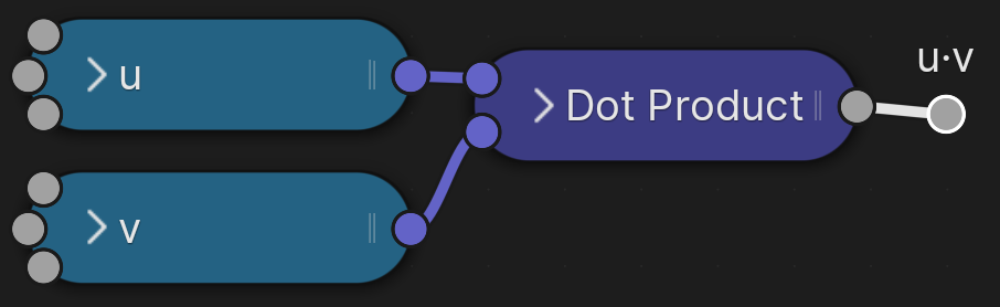
This is the fundamental piece of our matrix multiplication setup. The dot product tells us how long the piece of v is, that is parallel to u (or, in fact, vice-versa). So it’s going to be the coordinate of v that follows u.

However, to correctly multiply matrices, because the procedure asks us to “multiply rows by columns”, but our matrices are given in columns, we actually first need a way to swap columns and rows. Thankfully, that’s exactly what the Transpose of a matrix M^⊤ is all about:

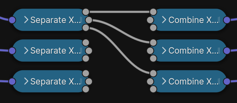
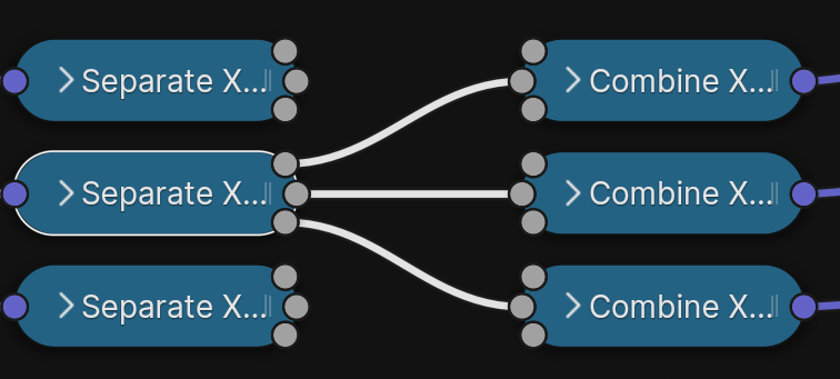
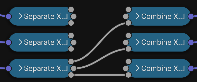
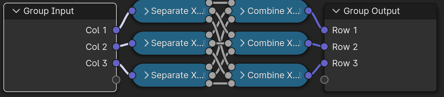
M^⊤, the Matrix Transpose, turning columns into rows

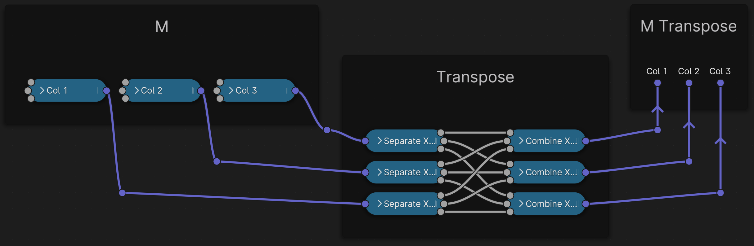
This is very simple to construct. Here just the individual strands starting from one node each:

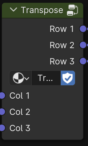
I recommend putting it in a group as we’ll need it a bunch:

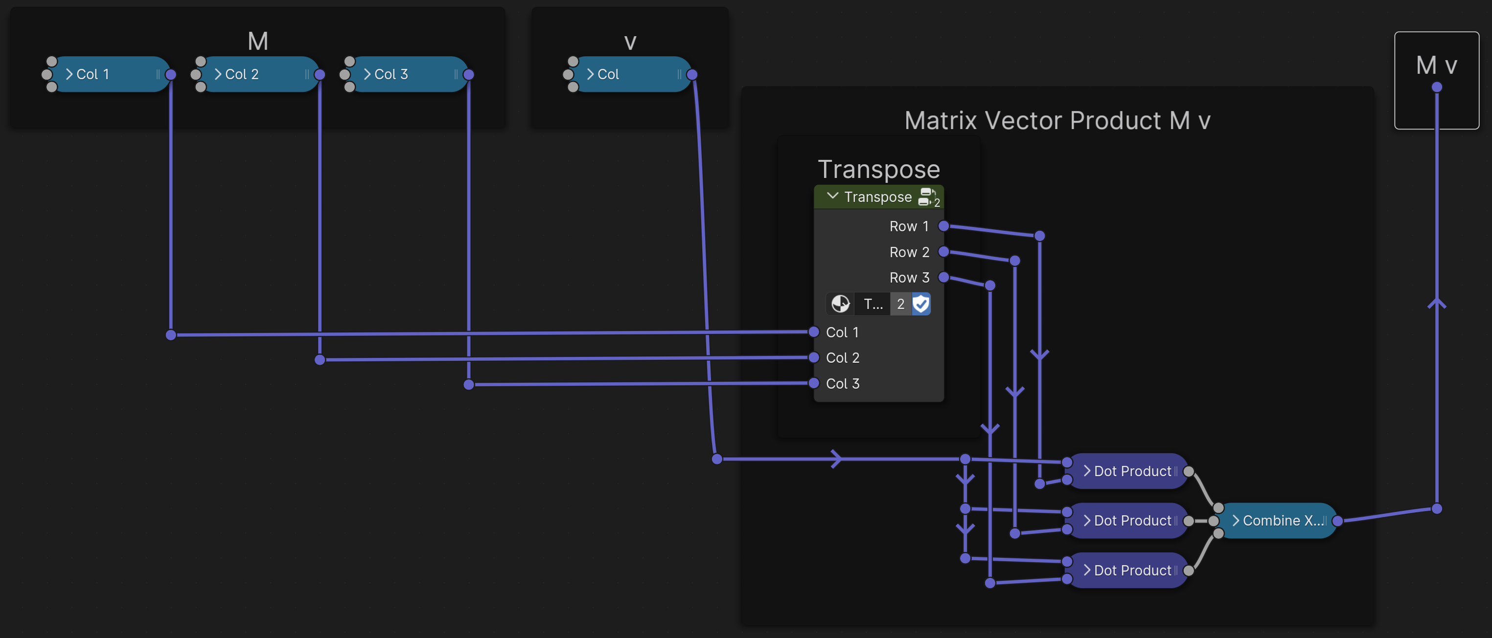
Now that we have that, we can complete our Matrix products:

M v — a Matrix applied to a column vector

M N — a Matrix applied to a Matrix

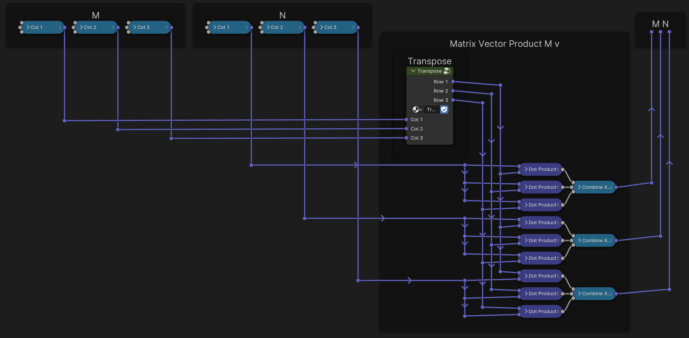
These two are going to be the main operations you’d like to use at any given time, so it’s a good idea to also turn both of these into a group.

However, it’s also going to be important to have the ability to invert matrices in order to undo whatever transformation you made.

---

The inverse of a matrix is the one that, multiplied with the original matrix, turns into 𝟙.
In particular, if you have these two matrices:

M = [u1 u2 u3]
N = [v1 v2 v3]

the various products
u_i^⊤v_j
ought to yield either 0 (off-diagonal) or 1 (diagonal):

⎡u₁^⊤⎤
⎢u₂^⊤⎥[v₁ v₂ v₃] = 𝟙
⎣u₃^⊤⎦

For instance,
u₂^⊤v₃
is supposed to be 0, because the subscripts don’t match up, whereas
u₁^⊤v₁
is supposed to be 1.

We therefore need to find a vector u₁ that is normal to both v₂ and v₃. (and so on)

As luck would have it, there is a simple operation that does this: The cross product. So let’s define:

u₁ = v₂ × v₃
u₂ = v₃ × v₁
u₃ = v₁ × v₂

and with that,

⎡(v₂ × v₃)^⊤⎤
⎢(v₃ × v₁)^⊤⎥[v₁ v₂ v₃]
⎣(v₁ × v₂)^⊤⎦

is going to be a matrix that is 0 in all off-diagonal entries.
However, at this point the three diagonal entries

(v₂ × v₃)^⊤v₁
(v₃ × v₁)^⊤v₂
(v₁ × v₂)^⊤v₃

could be anything, so we have to rescale by this.
It turns out, that no matter what, these three combinations turn out to be the exact same:

(v₂ × v₃)^⊤v₁ = (v₃ × v₁)^⊤v₂ = (v₁ × v₂)^⊤v₃

so we only actually need one of them. Let’s just choose the first one. This is also called the Determinant det(M) of the matrix M. Since you’ll have to divide by this to get to a unit matrix, if the determinant is 0, the result will be undefined. So the determinant determines whether any given matrix is actually invertible.
In fact, it captures the volume spanned by the three vectors [v₁ v₂ v₃]. If the determinant det(M) is 1, that means any object you send through that matrix will have constant volume. It might get squished in one direction but it’ll have to inflate in the other two. And if the determinant is negative, that means you’ll mirror the object on top of the other transformations.

But anyway, so what we have to do for the full inverse M = N^-1 is this:

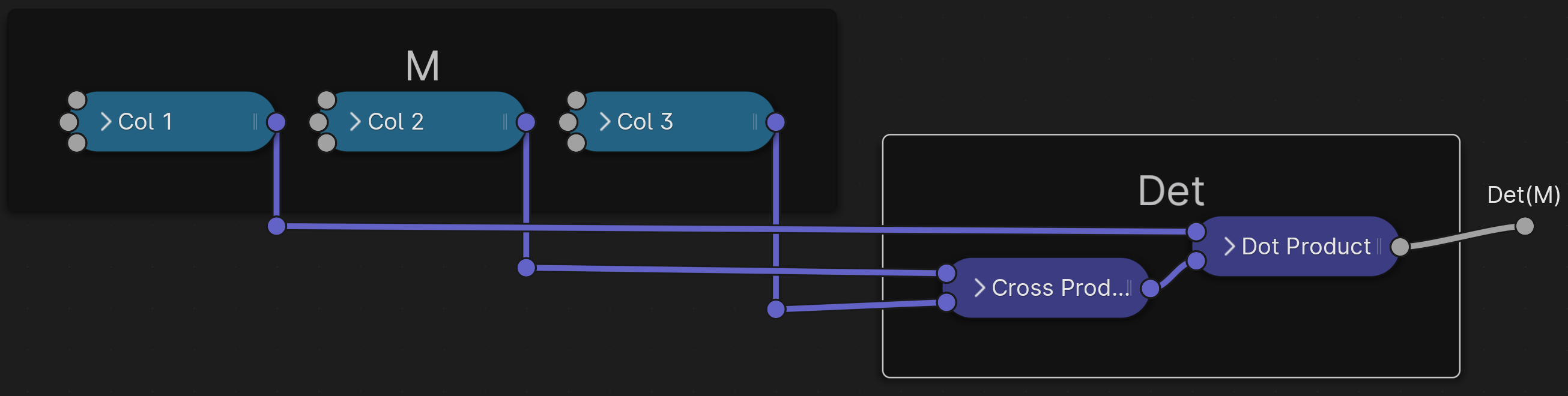
• find the determinant of the matrix N:
  Det(N) = (v₂ × v₃)^⊤v₁
• build the other cross products:
  u₁ = v₂ × v₃
  u₂ = v₃ × v₁
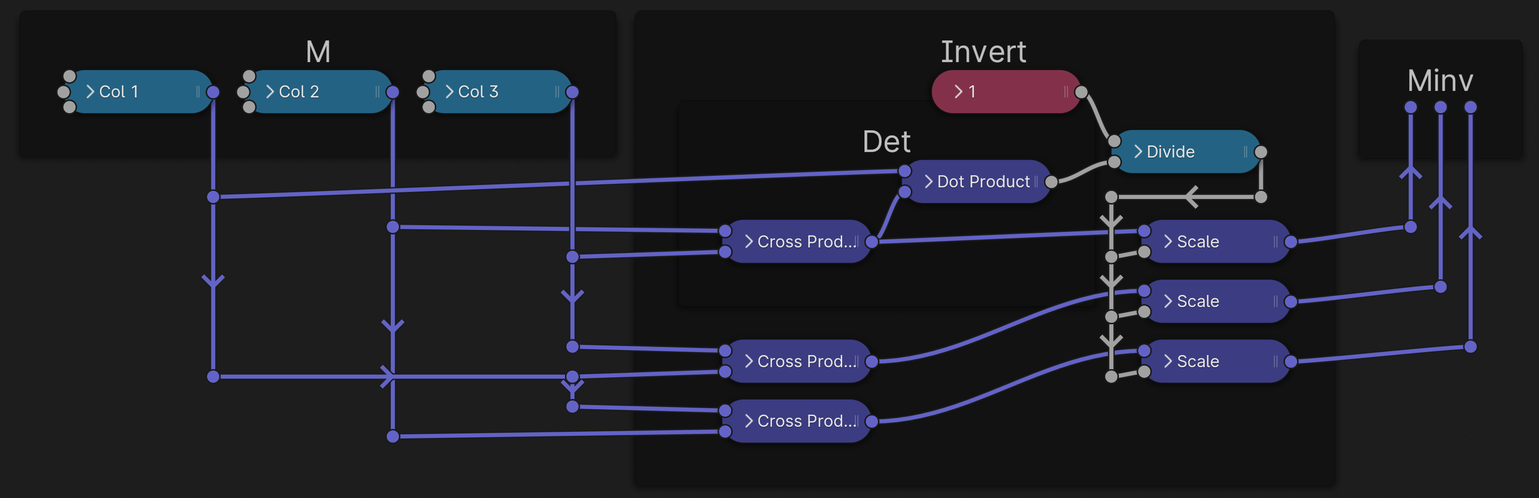
  u₃ = v₁ × v₂
• N^-1 = [v₂ × v₃, v₃ × v₁, v₁ × v₂] / ((v₂ × v₃)^⊤v₁)

Although matrix multiplication is not commutative (so M N isn’t always the same as N M), the inverse is the same for both sides. So that completes our inverse matrix.

In nodes that looks like this:

Det(M) — the determinant of Matrix M.

M^-1 — the inverse of M

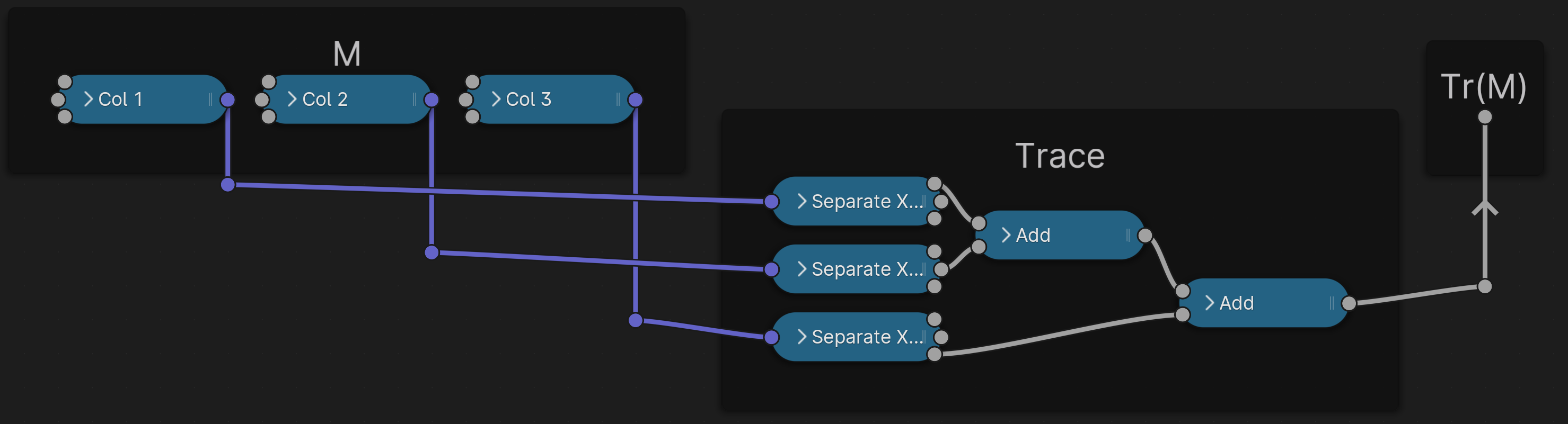
Finally, an important matrix invariant that often comes up is the Trace of the matrix. This simply is the sum of the diagonal entries:

---

Example application:

I constructed a randomized coordinate system:

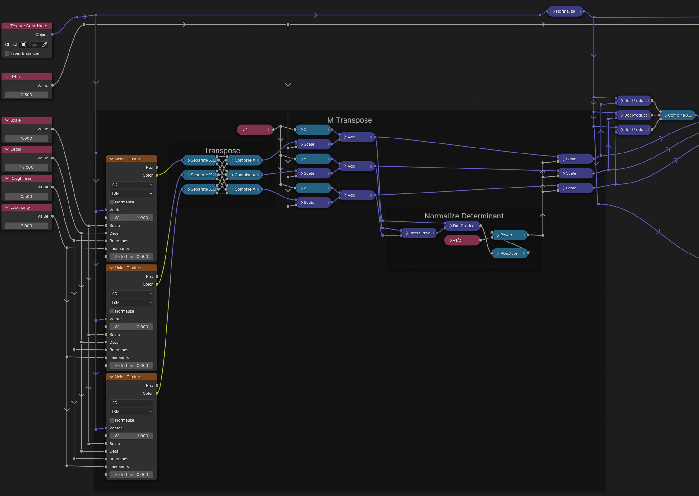
By adding position-dependent noise to 𝟙 and then normalizing the result such that the |determinant| is always 1.

This is like taking the regular XYZ coordinate grid (in object coordinates) and wiggling it a little bit, while ensuring local volumes remain constant.

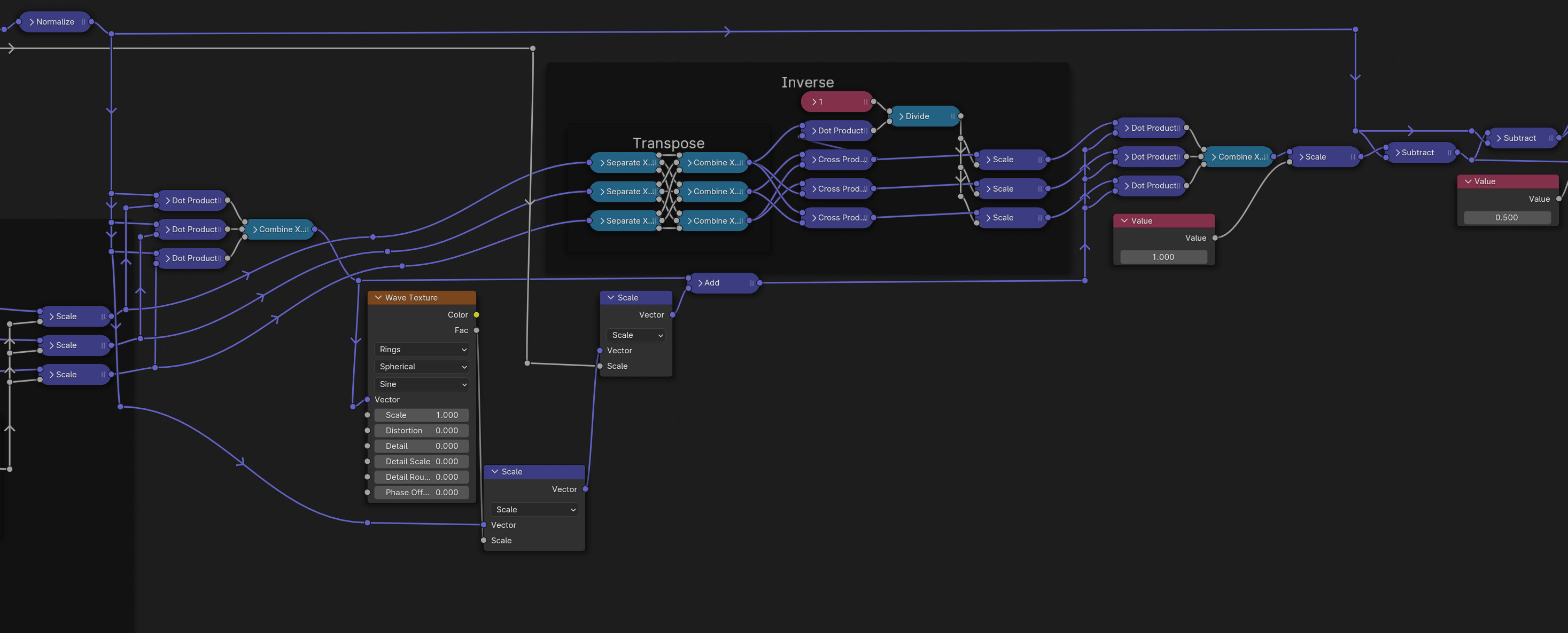
I then took that randomized coordinate grid and used it to drive a radial wave texture, and after, I transformed back using the Inverse block.

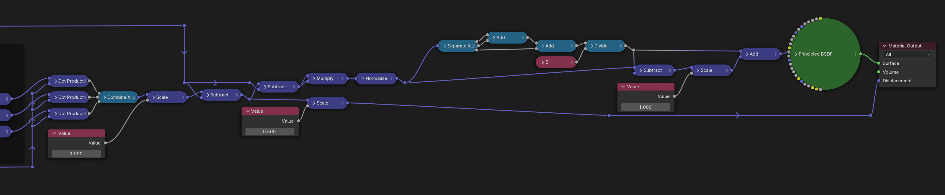
Finally, I just did some generic math to map the resulting texture into colors and displacement.

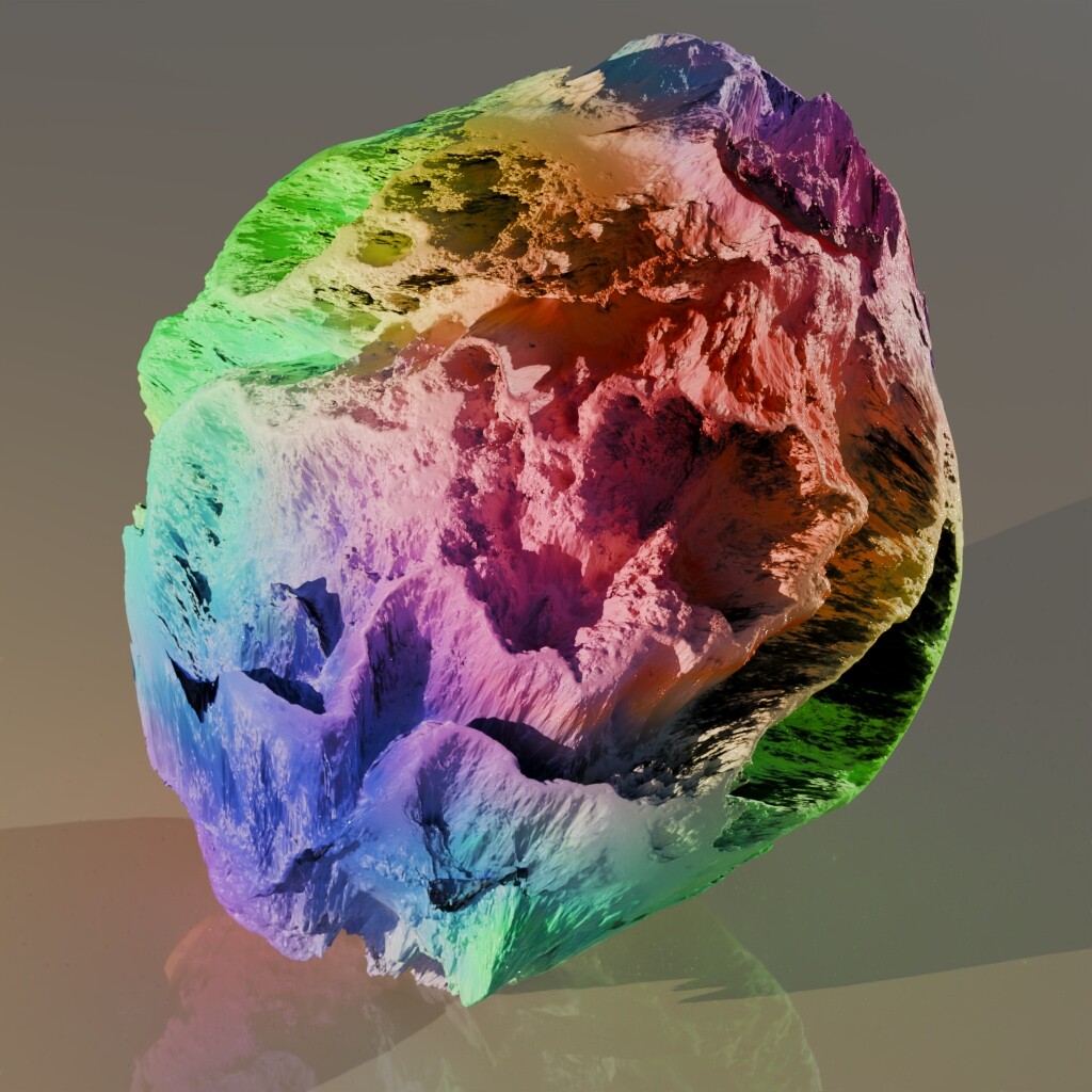
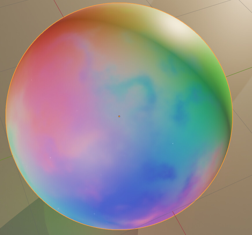
Applied to a sphere of radius 1, I get this result

Obviously there are a bunch of artefacts here from the severe distortion, but other than that it looks like an interesting texture to me. The result is very different from using the distortion slider on the wave texture.

The non-displaced version looks like this:

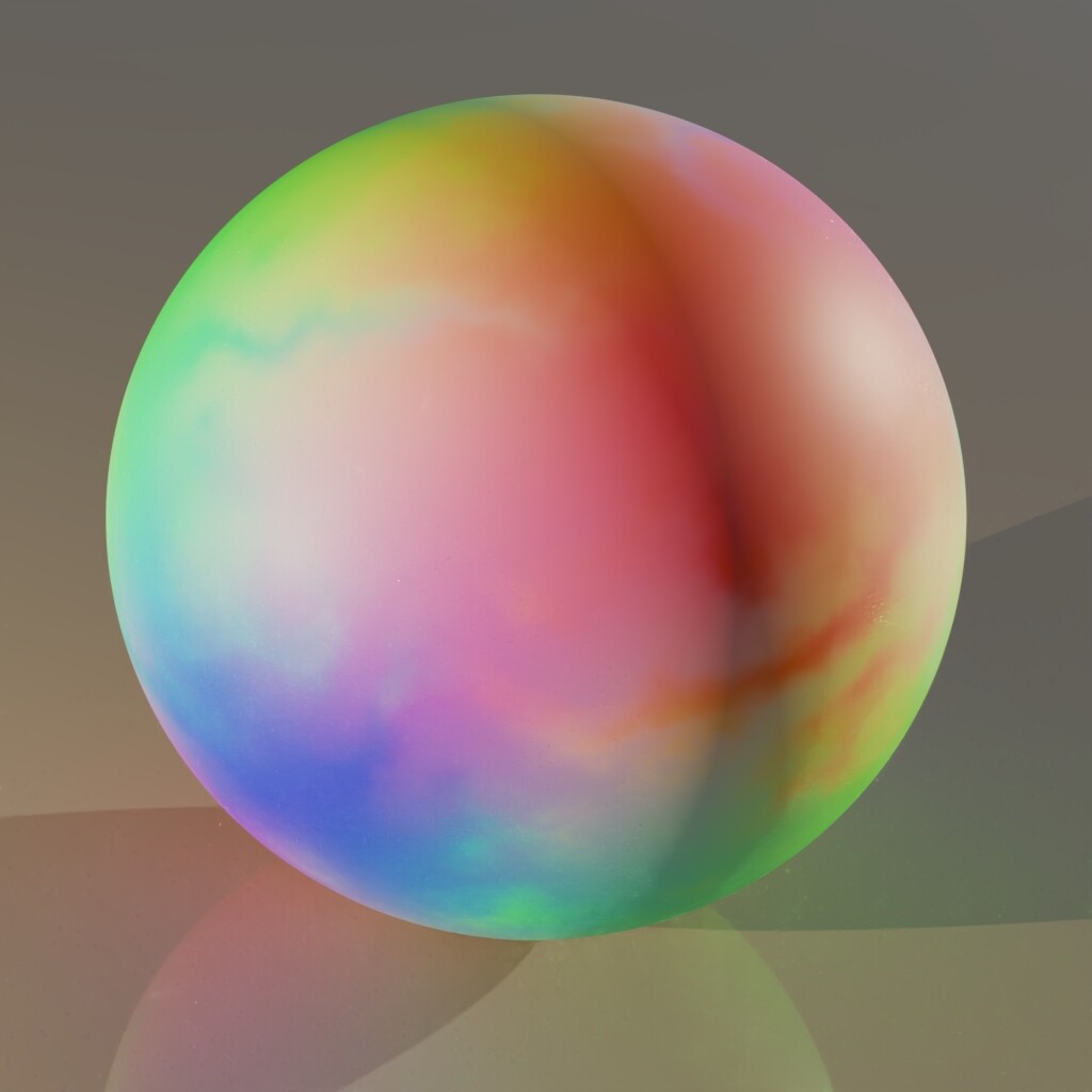
where you can see the formation of “ridges” or “tendrils” that definitely look quite distinct from the usual kinds of noise.

This is true from all sides:

[Secrop]

That’s what I miss from OSL!

I did wrote a bunch of nodes for 3x3 and 4x4 matrices math some years ago, but they were using hidden links to pass all the values from one node to another, and that option was removed in recent versions.

[kram10321]

Upgrading to 4x4 should work essentially the same except you have to route through an extra scalar and the inverse is gonna be more complicated (though similar)

[Secrop]

Yup. That’s why i was using hidden links… The visible connection was through a custom socket, but as the renderer wouldn’t understand it, the hidden links were where all data was being passed on.

[kram10321]

I’m not sure what you mean by hidden links. Like, a way to avoid excessive noodles?

It’d be amazing if we could just route through matrices directly, as a single noddle, rather than 3 (for a 3x3) or 8 (for a 4x4) etc.

[Secrop]

Before 3.4, if you would hide a socket from some node, its link wouldn’t be drawn. But the node_tree parser would still consider the link when reading the node_tree.

That way, the node would keep it’s sockets hidden (and links), except the MatrixSocket (which wasn’t doing nothing except being visible), and whenever the MatrixSocket was connected/disconnected to another node, a function was creating the links for the hidden sockets behind the scenes.

I have compiled the 4.1 version to still allow to hide sockets when linked, but I haven’t had the time nor the need to port those nodes to the 4.*.
I don’t know the current plans for nodes by the developing team, but I’d be happy to have that functionality back, even if only allowed for custom nodes.

[kram10321]

ah, seems like a really confusing concept. It’d be neat to have something like nameable noodles perhaps? Where you could either plug in noodles as you wish, or put in what amounts to attribute names instead.
That way you get your hiding functionality while also being clearer about what links to what, perhaps

[Secrop]

Something like this?
It was using the exact same logic…

[kram10321]

Oh nice! Not quite what I had in mind but that would also work.
This looks like kinda the opposite of a group node

[Secrop]

@kram10321

This looks like kinda the opposite of a group node

Hihi… An inside-out group node!

It also reminds me a bit the Repeat/Simulation nodes from GN…