Technical Report: Gradient Datamaps (Part II)
Part II: Clothing generator
2 comments before starting:
- I am changing the numbering scheme for Mutatis. Next version will be 1.2.281 instead of 1.281.2.
- This post is about a method to use gradient datamaps for clothing generation in Mutatis. In the following picture, the current version is on the left, and the improvement on the right.
I will now explain in detail how to do that.
II.1. Basics and first version
II.1.1. The idea
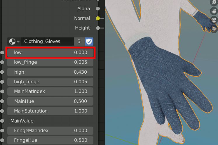
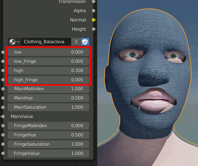
I wanted a simple way to generate simple clothing items (like underwear) that would always be sized and positioned properly on the base model. I remembered seeing a Youtube tutorial where the artist would duplicate the mesh to create a shirt (on a male model), and I figured that I could have something similar by keeping a duplicate mesh synchronized with the base mesh, and then use a procedural material with customizable transparency to create various shapes.
In Mutatis, the “synchronized with the base mesh” part is accomplished using what I call a proxyrig mechanism: there is a special proxyrig armature in which each bone is a child of a vertex of the base mesh. Unlike the Shrinkwrap modifier, the proxyrig bones stay at a predictable place relative to the unsubdivised* base mesh, regardless of what deformation is applied (shape key or armature).
* The Subdivision modifier causes the mesh surface to move unintuitively (up or down) relative to the unsubdivised surface. I will try to find a solution to that in the future.
To use this setup, I create:
- A linked duplicate of the proxyrig (pictured above: clothing proxyrig with small offset enabled).
- A duplicate of the base mesh without the shape keys and with the armature modifier set to the proxyrig linked duplicate.
I call this second object a proxymesh, and this technique is the basis for hair and clothing in Mutatis (it can also be extended to do other stuff, but more on that in future posts).
There are some apparent limitations with this method (the geometry of the clothing has to follow the geometry of the base mesh) but I thought it would be better than nothing as a starting point.
The hard part then was the customizable material. The relationship between long sleeves and short sleeves is obvious, and it doesn’t take long to notice that panties are kinda like very short trousers, and that bras are kinda like very skinny sleeveless shirts. In short, there might be a way to morph one clothing item into another based on the distance from the edges to some kind of wiry core.
I fiddled quite a bit with different techniques (the code is still buried in Mutatis 1.281.1, but I will clean it up for the new release). In the end, I settled on the following method:
- Create a shell, that is a simplified mesh where vertex weights help define a global gradient from the extremities to various “cores”.
- Position the vertices of the shell wrt to the clothing proxymesh, so that the core edges of the shell define natural separations between clothing items (not all the edges are core edges).
- Bake the interpolated weights into a texture appropriate for the clothing proxymesh (the picture below isn’t corrupted, the datamaps just look like that).
In the next sections I will focus on step 3 (generation of the gradient and region data + node setup to use the data).
II.1.2. Implementation in Mutatis 1.281.1 (without datamaps)
II.1.2.1. Generating the data
I don’t know if Blender allows baking vertex group weights into textures, so I decided to do the baking myself using the following steps:
- Use a dummy VertexWeightMix modifier on the shell (for some reason, this seems necessary for the script to access the subdivision-interpolated weights; see picture in previous section for the parameters).
- Use a Subdivision modifier on the clothing proxymesh.
- Rasterize the polygons (quad) of the clothing proxymesh into a 4k bitmap image.
- For each texel, compute the corresponding 3D point (the rasterization functions that I use allow for some kind of approximation; you can take a look at the script in Mutatis 1.281.1 if you are interested in the fine technical details).
- Use Blender’s Object.closest_point_on_mesh to get the closest point on the shell. This is used to determine both the interpolated weight (see below) and the clothing region id (face map index + 1).
- Use Blender’s mathutils.interpolate.poly_3d_calc to get the coefficients allowing to compute the interpolated point weight.
- Combine the weight and encoded region id into the texel color (red channel: weight, .
- Apply multiple dilations to the image in order to:
- Fill the holes left by the rasterization (the rasterization functions are a bit buggy).
- Add a margin around the islands (otherwise there are visual flaws when zooming out, perhaps because of lower texture LODs).
II.1.2.2. Node setup
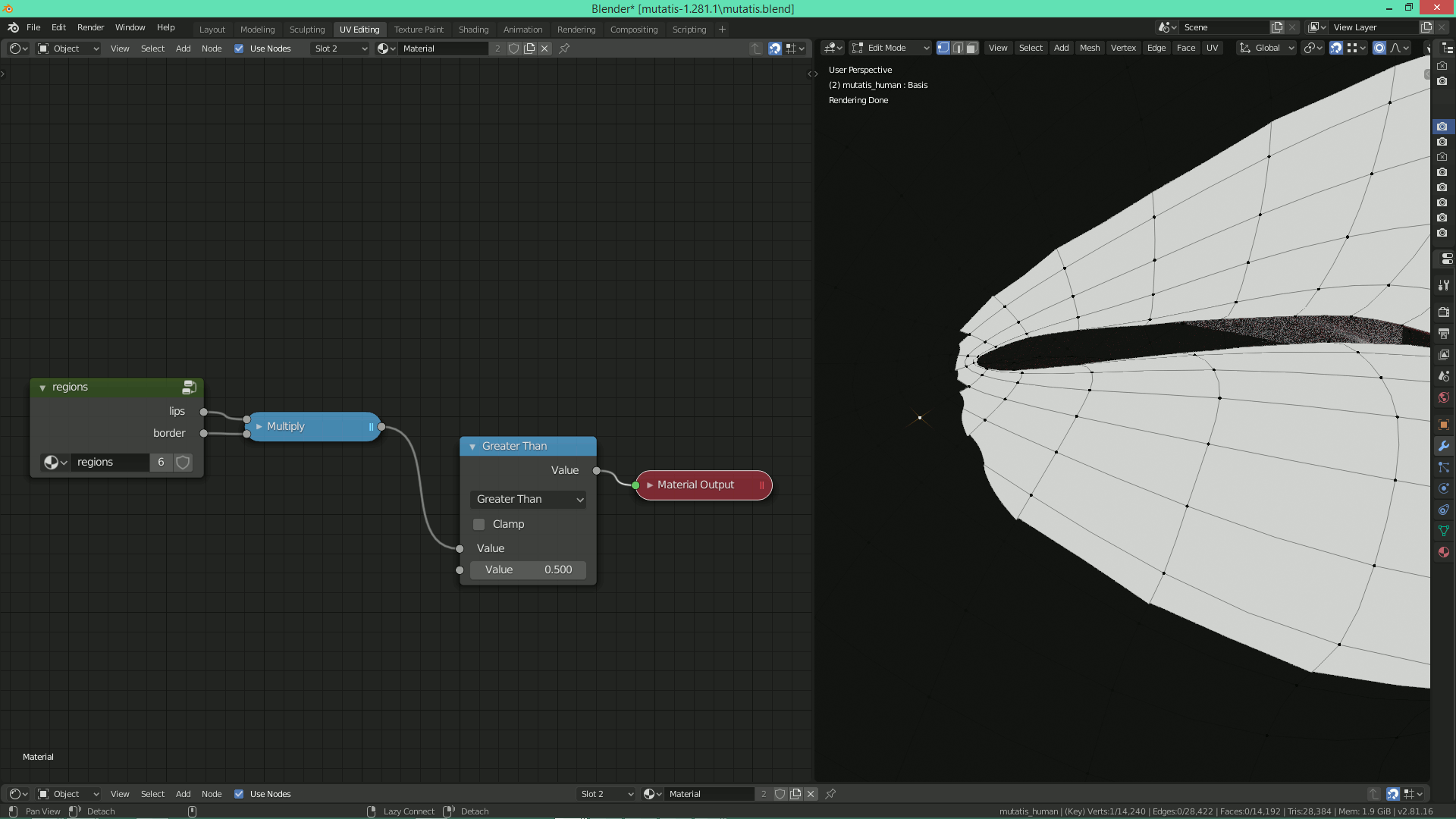
The node setup to use the image is straightforward: use the red channel to get the weight, and the blue channel to get the region.
Or at least it should be like that, but if you look at the ClothingRegions node group in Mutatis 1.281.1, I had to insert a UV quantization step before reading the region id, otherwise the borders between regions is not rendered properly in Cycles but only from a distance (close-up is fine).
I don’t know why this is necessary for Cycles but not Eevee. It could be a bug in Cycles, or it could be that I am doing something wrong but I don’t know what.
Either way, it won’t matter for 1.2.281 because I will probably be using datamaps as I explain in the next sections.
II.2. Planned improvements in Mutatis 1.2.281
II.2.1. Computation space and equation form
In Mutatis 1.281.1, some skin subregions are defined using simple datamaps (see previous post). The UV map “Data” is used for per-vertex/per-quad information storage, and the gradient computations are done using the UV map “UVMap”.
However, I defined the weights by hand with some intuitive expectation about the outcome, and this has implications which I did not realize at the time.
Consider for example the following configuration:
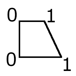
The 2 vertices on the left have weight 0, and the 2 vertices on the right have weight 1. Defining the weights this way, I expect to see a gradient from 0 to 1 that is going from left to right while still matching the trapezoidal shape of the quad.
But this means that the gradient in geometric space is non-linear (it is bilinear in this example).
In UVMap space it would be linear if the UV quad is a parallelogram, otherwise it would be non-linear.
This is important because if the gradient is non-linear, then there won’t be an exact solution to the system of equations (described in part I), which will result in visual deformations, as can be seen by looking closely at the last picture in part I.
There are several ways to deal with this, for example:
- Perform the computations in a space where the quads are guaranteed to be parallelograms.
- Use more complicated equations.
For option 1, the obvious candidate is UV Data space. I will probably use this for the skin in Mutatis 1.2.281.
Note: In the picture above, the remaining sharp angles near the corner of the mouth are due to me not defining the weights carefully enough, but I will try to fix this in the upcoming release.
However, this alone is not sufficient for the clothing because the gradient is more complicated, regardless of the computation space. So I will also use slightly more complicated equations.
In part I, I have talked about linear gradients which can be expressed with a simple formula ax+by+c. It is possible to turn things up a notch by considering bilinear gradients.
In the picture above, disregarding the exact symbolic coefficients, the overall form of the formula is:
Auv+Bv+Cu+D
This is convenient because it can be expressed as a dot product:
(C, B, D, A) . (u, v, 1, uv)
In short, I just have to append the product u*v to the homogeneous form (u, v, 1), and then let numpy.linalg.lstsq do the rest. The solution will simply have 4 coefficients instead of 3. Of course, the shader also has to be upgraded to take into account this additional element (more on that later).
Theoretically, it should be possible to keep extending the list with x^2, x*y^2, and so on, but it seems that I don’t have to go that far just yet (based on my observations).
II.2.2. Partitioned gradient datamaps
The main reason why I didn’t use gradient datamaps for the clothing in Mutatis 1.281.1 is that simple datamaps don’t provide a way to fit multiple regions inside a quad.
This wasn’t an issue for the skin because lips, palms, soles and genitals are all well separated.
However, the clothing is made of adjacent regions with hard borders over a global gradient that can suddenly change direction inside the quads (typically in the chest area).
Before proceeding, I simplify the problem by assuming that:
- At least one and at most two regions can be found inside a quad (this is not generally true, but the shell can be adjusted to limit the problematic cases).
- When there are more than one region inside a quad, the separation is a straight line splitting the quad in 2 parts (again, not generally true, but close enough).
- In each part, the gradient is approximately bilinear in UV Data space (same caveat as before).
With that in mind, the idea is to compute and store, at most, 2 gradients for each quad (one gradient for each region), and use the linear separation as a switch to select the correct region for the point being rendered in the shader.
II.2.2.1. Generating the data
This is very similar to the previous version, except that:
- The rasterization only produces one texel for each quad (disregarding subdivision, that means producing ~14000 texels, which fit inside a 128x128 image).
- The actual data is not a simple value but a more complicated structure requiring multiple images.
More precisely, I will use 4 RGBA images:
- The first 2 will hold the encoded coefficients for the (approx) bilinear gradients, one image for each region.
- The third will hold the encoded scales (see encoding in part I) and the encoded region ids (encoding/decoding a region id is simply dividing/multiplying by 32).
- The fourth will hold the encoded coefficients and scale for the linear separator.
Thus, for each quad, the following algorithm will produce 4 RGBA “texels” (in UV Data space):
-
For each “loop” (Blender terminology for topological half-edge or dart), determine a splitting point (I use dichotomic search with 16 steps). If there is no split, use the other end of the loop as default splitting point.
-
Pick 2 splitting points (prioritize real splits over default splits).
-
Use these 2 points to compute a linear separator in UV Data space.
This is easily accomplished with projective geometry by computing the cross product of the homogeneous coordinates of the 2 points:
sep_coeffs = (split1.u, split1.v, 1) x (split2.u, split2.v, 1)
-
Apply the separator (dot product) to place the vertices and splitting points into 2 groups:
- Group 1 contains both splitting points and all vertices with a positive dot product (vert.u, vert.v, 1) . sep_coeffs > 0
- Group 2 contains both splitting points and all vertices with a negative dot product (vert.u, vert.v, 1) . sep_coeffs < 0
A linear separator is identical in form to a linear gradients (3 coefficients), and the separation line can be visualized as a region of space where the corresponding gradient is 0, while each of the surrounding half-planes holds either positive or negative gradient values.
- Attribute a region id to each group (I just use the region id of the first vertex in each group).
- Compute the gradient coefficients of each group using the method described in part I with extended homogeneous coordinates: (u, v, 1, u*v)
- Encode the 3 sets of coefficients (gradients for both groups and separator) and store the encoded coefficients, scales and region ids as described earlier.
II.2.2.2. Node setup
The node setup does the following:
- Decode the 3 sets of coefficients (2 bilinear gradients, 1 linear separator).
- Apply each of these sets to the current location in Data space (dot product with extended homogeneous coordinates).
- Decode the 2 region ids and create a region mask for each (the mask here is the binary value of the equality with a region id provided as user input).
- Use the output of the linear separator as a switch to select a pair, either (gradient 1, region 1) or (gradient 2, region 2).
Steps 1 to 3 can be seen in the following picture:
Step 4 can be seen in the following picture:
The following pictures illustrate the various concepts that I have just presented on a part of the clothing proxymesh where a shell border between regions crosses through multiple quads.
Here is an isolated view of the shell:
In this color-coded view of the regions selected by the linear separator, the masking region id used as input is the one for the right arm, and region 1 and region 2 are defined independently for each quad as explained previously:
In this next picture, I overlay the band containing the upper values of the gradient in this region:
Finally, adding the textures and the other regions:
If you look closely, the supposedly linear separator seems “broken” in some of the quads. I am not completely sure, but this could be due to Blender’s triangulation:
II.3. Conclusion
In these last posts (part I and part II) I tried to explain the datamap technique that I use to approximate gradients in Mutatis’s shaders.
The advantages compared to a bitmap (traditional) 4k high precision gradient map are:
- No aliasing (staircase effect) regardless of the viewing distance.
- Reduced data file size (200 Mb → 500 kb).
The disadvantages are:
- Complexity of data generation and of node setup.
- Doesn’t work in Eevee (I don’t know why).
In addition to the improvements presented here, I am putting the finishing touches on a new clothing shell that should be able to hold 2 independent gradients. This will add a couple of (small) data files but it should then be possible to add more details to the clothing (like seams).